Roofline: The First Step of Any Performance Optimization
When MFU sits at 20%, most people open a profiler and hunt for a slow kernel. That often starts at the wrong layer. The first question is not which kernel is hot — it is which ceiling you are hitting: compute or memory bandwidth.
TL;DR
- Every GPU has two hard ceilings: peak FLOP/s and peak bandwidth. Arithmetic intensity
I = FLOPs / Bytesdecides which one binds first. - MFU answers “are we compute-bound?” for training. MBU answers “are we bandwidth-bound?” for decode. Both are Roofline ratios, not vibes.
- Shape matters more than op name: the same
matmulcan be compute-bound atM=N=K=8192and memory-bound atM=1. That is why training and decode feel like different worlds. - Count MFU/MBU by instrumentation (
FlopCounterMode+ bytes), not PaLM6PT— that formula is an LLM shortcut. ResNet / ViT work the same way as any othernn.Module. - Model-level Roofline is useful when traffic is homogeneous (decode, dense training GEMMs). It is misleading when time is dominated by a mix of memory-bound and compute-bound ops — then go per-op, then profiler.
- Reproducible Modal measurements (ops, LLM decode/train sweeps, ResNet/ViT MFU·MBU) live in this page bundle; code in
playground/roofline_modal.py.
The Most Expensive Mistake
The costly failure mode in performance work is not missing the optimal kernel. It is optimizing in the wrong direction.
A recurring upgrade story:
Dense training on A100 at ~45% MFU. Move to H100 expecting ~3× from peak BF16. Wall-clock improves ~1.5×; MFU falls to ~32%. The team blames NCCL, CUDA, or “bad kernels.” The real change: the ridge point moved. Ops that sat on the A100 plateau were pushed onto the H100 slope.
Hardware keeps rewriting the binding constraint. Roofline is the cheapest way to see that before you spend a week in Nsight.
The Model in One Page
Roofline (Williams, Waterman, Patterson, CACM 2009) says:
Achieved performance ≤ min(
I × PeakBW,PeakFLOPS).
Iis mostly an algorithm/shape property (and precision). Moving the same GEMM to a new GPU does not changeI; it moves the roof around the point.- Left of
I_peak: memory-bound — raise reuse / fuse / cut traffic. - Right of
I_peak: compute-bound — Tensor Cores, lower precision, better tiling / shapes. - Near
I_peak: both matter; pick by ROI.
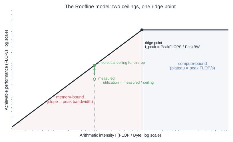
Utilization is simply measured rate ÷ the roof height at that I. A profiler reports milliseconds; Roofline asks whether those milliseconds were spent computing or waiting on DRAM.
Classic FP32 intensities:
| Operation | FLOPs | Bytes | I |
|---|---|---|---|
| SAXPY | 2N | 12N | 0.17 |
| Dot | 2N | 8N | 0.25 |
| Square GEMM N×N | 2N³ | 12N² | N/6 |
GEMM’s I scales with N. Large matmuls are structurally compute-bound; elementwise ops are structurally memory-bound. That is not a failed optimization — it is the algorithm.
The Ridge Keeps Moving Right
Dense datasheet peaks (no sparsity):
| GPU | Peak BF16 | Bandwidth | I_peak (BF16) |
|---|---|---|---|
| V100 SXM2 | 125 TFLOPS | 900 GB/s | ~139 |
| A100 SXM 80GB | 312 TFLOPS | 2039 GB/s | ~153 |
| H100 SXM | 989 TFLOPS | 3.35 TB/s | ~295 |
| H200 SXM | 989 TFLOPS | 4.8 TB/s | ~206 |
| B200 | 2250 TFLOPS | 8 TB/s | ~281 |
| GB200 NVL72 | 2500 TFLOPS/GPU | 8 TB/s | ~312 |
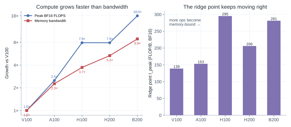
Since V100, BF16 compute grew ~18× while bandwidth grew ~8.9×. The ridge moved from ~139 to ~295 on H100. More of the operator zoo sits on the slope every generation.
That is the shared story behind FlashAttention, aggressive fusion / torch.compile, and FP8 GEMMs: raise effective I or stop pretending low-I work can drink peak FLOPS.
FP8 makes the ridge worse for non-GEMM work: H100 FP8 peak ~1979 TFLOPS ⇒ I_peak(FP8) ≈ 591 with the same HBM. Elementwise ops get shoved further left. FP8 is a GEMM/tooling bet, not a free lunch for the whole graph.
How to Score: MFU and MBU
The definitions are model-agnostic. The counting method is what people get wrong.
Do not start from PaLM’s 6·P·T. That is a shortcut for dense Transformer LLMs, not a universal FLOP counter. ResNet, ViT, U-Net, diffusion backbones — none of them owe you a closed form. The portable method is instrumentation:
- FLOPs —
torch.utils.flop_counter.FlopCounterMode(or fvcore). Run the real forward, or forward+backward, under the same autocast you use in production. - Bytes — either DRAM bytes from Nsight Compute, or a module-boundary estimate: for every leaf module, charge parameter reads + input/output tensor sizes. The estimate over-counts when activations stay in cache / get fused, and under-counts workspace invisible at boundaries. It is still the right default when you do not have
ncu. - Time — median CUDA events around the same region you counted.
| |
LLM special case (optional shortcut)
For dense Transformer LLMs only, FLOPs/step ≈ 6·P·T (Kaplan / Chinchilla): forward 2PT, backward 4PT. Long sequences need the attention term or you understate FLOPs and inflate MFU:
| |
Public LLM ballparks still use this shortcut: PaLM 540B ~46% on TPU v4; Llama-2 70B ~40–45% on A100. Below ~20% on a healthy dense LLM job, look for data / launch / communication first.
MFU vs HFU: HFU counts checkpoint recompute in the numerator. HFU = “is the GPU busy?”; MFU = “useful model work.” Ask whether a quoted “60% MFU” includes recompute.
Decode → MBU (LLM serving)
Batch-1 BF16 decode is dominated by streaming weights. Llama-70B on H100:
That bound is physical. Speculative decoding, continuous batching, and quantization change the bytes or the effective batch — they do not violate Roofline. Good serving stacks often land in the 60–80% MBU band; below ~40% usually means launch / CPU / graph overhead.
Operator Intensities (Keep This Table)
Horace He’s framing still stands: time splits into compute, memory, overhead. Roofline covers the first two. Overhead (eager launches, Python, host sync) is a third wall — high when both MFU and MBU are low.
| Operator | I (BF16, approx.) | On H100 | Lever |
|---|---|---|---|
| Elementwise | 0.5–1.5 | memory | fuse |
| RMSNorm / Softmax | ~1 | memory | fused kernels |
| Vanilla attention | tens | memory | FlashAttention |
| FlashAttention | hundreds–thousands* | near/on plateau | already the right direction |
| GEMM 4096³ | ~10³ | compute | TC alignment, FP8 |
| GEMM M=1 (decode) | ~1–2 | memory | batch, quantize |
| Embedding | ~0 | memory | cache / low-precision storage |
*Depends on how you count SRAM-resident intermediates; the point is FA collapses HBM traffic from O(S²) to O(S) at nearly constant FLOPs — “raise I” and “cut memory traffic” are the same move.
The two GEMM rows are the root of “training feels compute-bound, decode feels memory-bound”: same op family, different shapes, different I.
Experiments
All scripts: playground/roofline_modal.py, figures: playground/roofline_figures.py.
Setup. Modal free tier here → A10 / A10G-class GPUs, not H100. Op sweep figures use an A10G datasheet roof (70 TFLOPS BF16, 600 GB/s, I_peak ≈ 117). Decode/train/CV sweeps landed on an A10 (125 TFLOPS BF16, same 600 GB/s, I_peak ≈ 208). The shapes transfer; only the ridge moves on H100. Timing is median CUDA-event walls. Per-op FLOPs/bytes are analytic; CV FLOPs come from FlopCounterMode; CV bytes from leaf-module IO (+ bwd weight/grad traffic for train). BF16 matmul uses FP32 accumulation where relevant.
Measurement idea (not the full harness):
Per-op: theory shows up on a stopwatch
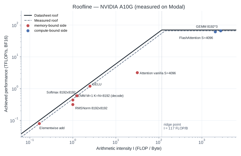
| Op | I | Achieved | Read |
|---|---|---|---|
| memcpy ceiling | — | 472 GB/s | ~79% of 600 GB/s |
| GEMM 8192³ | 2731 | 65.9 TFLOP/s | ~94% of 70 TFLOPS |
| Elementwise add | 0.17 | 477 GB/s | on the slope |
| Decode GEMV M=1 | ~1 | 0.44 TFLOP/s, 438 GB/s | 73% MBU, not a “slow kernel” |
| Vanilla attn S=4096 | ~32 | 3.2 TFLOP/s | HBM-bound scores |
| FlashAttention S=4096 | ~2048 | 61.4 TFLOP/s | ~88% of peak; ~19× wall-clock |
Three takeaways:
- Memory-bound ops pin bandwidth and refuse FLOPS. Tuning
addis theater; fusion is the only lever. - Decode GEMV vs square GEMM is ~150× in TFLOP/s for the same
matmulAPI. Shape, not kernel quality. - FlashAttention moves the same FLOPs from the slope onto the plateau by cutting bytes.
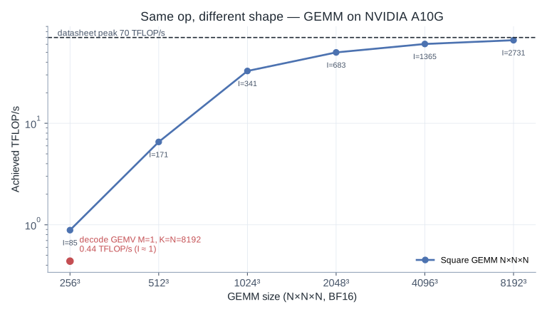
Even within “square GEMM,” 256³ is ~1% of peak; the roof only appears once tiles fill the machine. Whitepaper peaks assume shapes the library likes.
Model-level: when averaging is honest
A whole-model “average I” is dangerous when GEMMs dominate FLOPs but norms/softmax dominate time. Then Roofline must be applied per hot op, and a profiler tells you which ops are hot.
It is honest when traffic is dominated by a single pattern:
Decode. One step reads weights once (~2P bytes BF16) and does ~2P·B FLOPs:
| |
Batch is intensity. Throughput should rise almost linearly until B ≈ I_peak, then flatten. That knee is the critical batch — a number a single profile cannot invent.
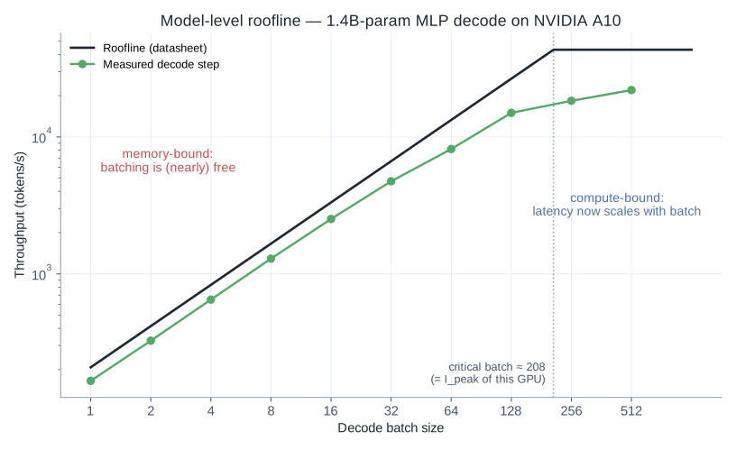
On A10 (critical batch ≈ 208), 1.4B MLP decode:
- Batch 1: 166 tok/s vs ~208 tok/s bandwidth ceiling (~80% MBU).
- 1→128: ~90× throughput; step time 6.0→8.5 ms — batching is nearly free.
- 128→512: 4× batch → ~1.5× throughput; latency climbs — past the ridge.
Training (LLM-shaped stand-in). For this MLP, the LLM shortcut 6P·T is intentional — same accounting as a dense Transformer without attention. Weight traffic ≈ 6P bytes BF16 (fwd read, bwd read, grad write):
| |
Real LLM training uses huge T, so the aggregate step sits on the compute roof — which is why MFU is the right headline metric. Same model, same GPU, sweeping T:
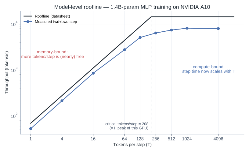
- T=1: 53 tok/s — ~3× slower than decode batch=1; three weight traversals vs one.
- 1→128: ~97× throughput; step time barely moves — still on the slope.
- 1024→4096: plateau ~8k tok/s, ~70 TFLOP/s → ~56% MFU on this A10. Production
Tis far larger; you live on the plateau and ask how close, not which wall.
Aggregate compute-bound does not mean every op is. Norms and softmax still sit on the slope; that is why fusion and FlashAttention still matter inside an “MFU-healthy” train job.
CV models: MFU/MBU without a closed form
ResNet-50 and ViT-B/16 have no honest 6PT. The CV sweep (::cv) uses the portable recipe above: FlopCounterMode for FLOPs, leaf-module IO (+ bwd weight/grad bytes for train) for traffic, CUDA-event medians for time. FP32 master weights, BF16 autocast — the same pattern most training stacks use.
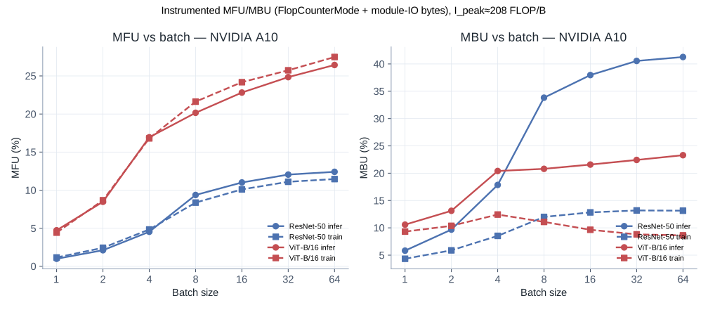
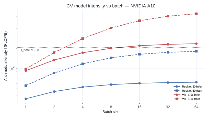
At batch 64 on A10 (I_peak ≈ 208):
| Model | Phase | I | MFU | MBU | img/s |
|---|---|---|---|---|---|
| ResNet-50 | infer | 63 | 12% | 41% | 1896 |
| ResNet-50 | train | 182 | 12% | 13% | 589 |
| ViT-B/16 | infer | 236 | 26% | 23% | 941 |
| ViT-B/16 | train | 664 | 28% | 9% | 325 |
What to read:
- ResNet inference sits left of the ridge (
I ≈ 63 < 208). MBU rises with batch and tops out near 40%; MFU stays low. This is a bandwidth-leaning CNN: BN/ReLU/small convolutions keep average intensity modest. Fusing and channels-last / efficient BN matter more than “more Tensor Cores.” - ViT training crosses the ridge (
I ≈ 664). MBU falls while MFU climbs — classic compute-side behavior as matmul-heavy blocks amortize weight traffic over larger batches. - Both MFU and MBU are modest in absolute terms on this eager torchvision path. That is Shape C contamination (Python / launch / unfused eager graph), not a claim that ResNet is “broken.”
torch.compileor a fused training stack would move the points up without changing the relative ResNet-vs-ViT story. - Same method, any model. Swap in U-Net or a detector head; the counter does not care. LLM
6PTis convenience, not a prerequisite for Roofline.
Roofline vs profiler. Roofline is forward-looking: ceilings, critical batch / critical T, whether an idea can help. A profiler is backward-looking: where time went in the run you already made. Order: napkin Roofline → instrumented MFU/MBU → per-op Roofline → profiler.
A Playbook
| |
Canonical shapes:
| Shape | MFU | MBU | Typical fix |
|---|---|---|---|
| A | high | low | precision, TC, MoE/sparsity |
| B | low | high | fusion, FA, KV reuse, quant |
| C | low | low | compile, graphs, bigger work units |
Shape C looks like Horace He’s timeline: idle → burst → idle.
Traps
- Maximizing MFU ≠ maximizing useful tokens/s. Padding to a “fast” shape can raise MFU while lowering effective throughput.
- Two roofs is a teaching model. Hierarchical Roofline (L2, shared memory, NVLink, IB) matters for multi-GPU.
Iindependent of batch is false for GEMM. DecodeM=1collapsesI.- Whitepaper FLOPS are conditional. Dense vs sparse (A100 312 vs 624; H100 989 vs ~1979), TC on, aligned shapes. The GEMM sweep above is the shape condition made visible.
- High MFU does not retire MBU. Training headlines MFU; decode headlines MBU. Use both to avoid cargo-culting the wrong ratio.
Closing the H100 Story
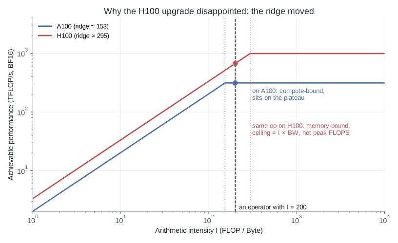
A100 I_peak ≈ 153, H100 ≈ 295. An op at I = 200 sits on the A100 plateau and on the H100 slope. Compute rose ~3.2×; bandwidth only ~1.65×. The fix was not “find the NCCL bug” — it was raising effective I (FlashAttention, larger batches, FP8 GEMMs) to the right of the new ridge.
Roofline does not name the bug. It names the wrong hunt.
What This Is Not
Roofline will not debug imbalance across ranks, dynamic-shape recompile storms, or PCIe/CPU feed issues in detail. Those need timelines. Use Roofline so you open the profiler with a hypothesis, not a panic.
References
- Williams et al., Roofline, CACM 2009; LBNL Roofline; NVIDIA DL Performance Guide
- Chowdhery et al., PaLM; Kaplan et al., Scaling Laws; Hoffmann et al., Chinchilla
- Databricks / MosaicML, LLM Inference Performance Engineering
- Horace He, Making Deep Learning Go Brrrr; Dao et al., FlashAttention / FA-2