Pipeline Parallelism from First Principles: Why GPipe Split the Batch
Pipeline parallelism starts with a useful accident: a Transformer is already a chain. If one GPU cannot hold the whole stack, put consecutive blocks on consecutive GPUs and send activations across stage boundaries.
That solves capacity. It does not solve throughput. A naive layer split turns an expensive cluster into a queue where most devices wait. GPipe’s contribution was to make the queue busy by slicing the mini-batch into micro-batches and recomputing activations instead of storing everything (arXiv:1811.06965).
Modern pipeline systems add 1F1B schedules, interleaving, PipeDream-style asynchrony, and zero-bubble tricks. Those are refinements. The core mechanism is still the GPipe triangle: bubble, activation memory, and stage balance.
TL;DR
- Pipeline parallelism partitions the layer stack. It is different from tensor parallelism, which partitions the math inside a layer.
- Naive layer-wise model parallelism fits more layers but has bubble fraction
(K - 1) / KforKstages. AtK = 8, 87.5% of device-time is idle. - GPipe splits one mini-batch into
Mmicro-batches. Its flush schedule reduces the bubble to(K - 1) / (K + M - 1)(arXiv:1811.06965). - Rematerialization stores stage-boundary activations and recomputes local activations during backward. It trades FLOPs for HBM.
- 1F1B schedules reduce activation residency. PipeDream trades clean synchronous semantics for weight staleness (arXiv:1806.03377). Zero-bubble schedules try to fill idle slots with weight-gradient work.
- The production question is not “GPipe or not.” It is: how deep can the pipe be before bubbles, imbalance, and activation traffic eat the win?
- Reproducible figures for this post:
playground/llm_training_series_figures.py.
1. What Pipeline Parallelism Partitions
Let a model have L layers and K pipeline stages. A balanced partition gives each stage about L/K layers:
Forward sends activations from stage i to stage i + 1. Backward sends activation gradients in reverse. Parameters stay on the stage that owns the layer.
That is the capacity win. Each GPU stores only its local layers, local optimizer state, local gradients, and the activations it needs for its stage. If a model fails because the full stack does not fit, pipeline parallelism is the natural partition.
The cost is that a chain has dependencies. Stage 3 cannot run micro-batch j until stage 2 has produced its activation. The schedule decides whether those dependencies leave GPUs idle.
2. Naive Layer Splitting Fits, Then Waits
The direct schedule sends one mini-batch through all stages, then sends its backward pass back.
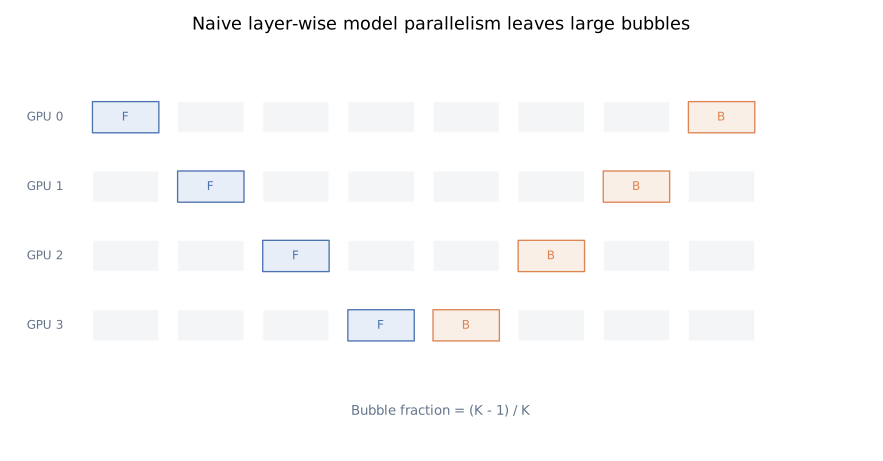
Only one stage works at the beginning of forward. The pipe fills slowly. Then only one stage works at the end of backward. For one mini-batch, assume every stage has equal time t_f + t_b.
The math is not subtle:
K = 2: 50.0% idle.K = 4: 75.0% idle.K = 8: 87.5% idle.
This is why “just split layers across GPUs” disappoints. Capacity improves while utilization collapses.
Naive splitting also leaves activation memory unsolved. For local batch N, hidden width d, and local depth L/K, stored activations scale roughly as:
| |
That is smaller than the full stack, but it is still proportional to local depth and batch. Increasing global batch to use more GPUs can push the memory problem right back onto each stage.
3. GPipe’s Move: Micro-Batch the Mini-Batch
GPipe keeps synchronous mini-batch semantics but feeds the pipeline with M micro-batches.
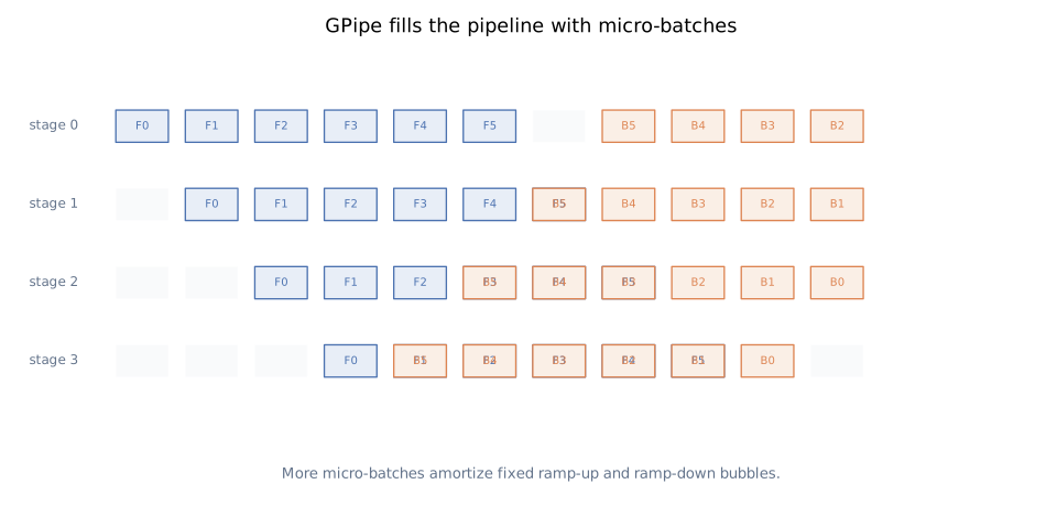
Definitions:
K: pipeline stages.M: micro-batches inside one mini-batch.N: original mini-batch size.N/M: per-micro-batch size.
Stage 0 starts micro-batch 0, then starts micro-batch 1 while stage 1 processes micro-batch 0. Once the pipe is warm, all stages work on different micro-batches from the same mini-batch.
For GPipe’s synchronous flush schedule, the bubble fraction becomes:
| |
For K = 8:
M = 1:7/8 = 87.5%.M = 8:7/15 = 46.7%.M = 32:7/39 = 17.9%.
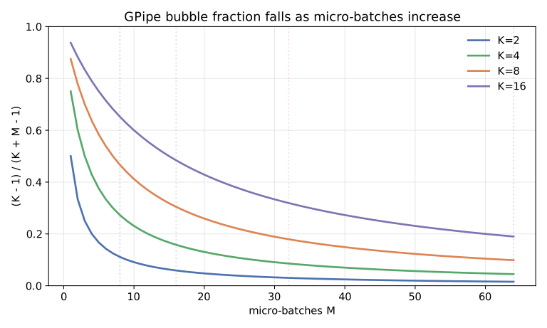
The direction is clear: more micro-batches amortize the fixed fill/drain bubble. The limit is also clear: micro-batches eventually become too small. GEMMs shrink, kernel launch overhead matters, normalization/statistics edge cases appear, and activation bookkeeping grows.
The GPipe paper reports near-linear model-size scaling on Transformer workloads because the stack is regular and partitions cleanly (arXiv:1811.06965). That result is not a magic property of pipelines. It is a property of balanced stages with enough micro-batches.
4. Synchronous Flush Semantics
GPipe accumulates gradients over the M micro-batches and applies one optimizer step for the original mini-batch.
The benefit is clean:
- Every micro-batch in the mini-batch sees the same parameter version.
- The update matches ordinary synchronous mini-batch training, aside from numerical ordering.
- Optimizer, checkpoint, and loss-scaling semantics remain easy to reason about.
The cost is the flush. GPipe runs all forwards, then all backwards, then updates. The pipeline must drain before the next mini-batch can use updated weights.
That cost explains later schedules:
- 1F1B: once warm, each stage alternates one forward and one backward. This reduces activation residency because backward starts before all forwards finish. Megatron-LM’s pipeline implementation relies on this family of schedules at scale (arXiv:2104.04473).
- PipeDream: allows asynchronous pipeline execution and manages multiple weight versions, trading higher utilization for weight staleness and more complex semantics (arXiv:1806.03377).
- Interleaved 1F1B: splits one physical device into multiple virtual pipeline stages to reduce bubble and improve balance when communication allows it (arXiv:2104.04473).
- Zero-bubble schedules: split backward into input-gradient and weight-gradient work so otherwise idle slots can compute weight gradients. The point is not zero cost; the point is moving useful work into bubble time.
GPipe remains the best first model because it makes the dependency graph visible.
5. Activation Checkpointing: Trade FLOPs for HBM
Micro-batches reduce idle time. Rematerialization reduces activation memory.
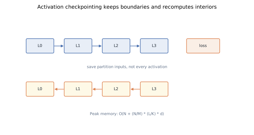
Backward needs forward activations. The naive plan stores every intermediate tensor produced by every local layer for every micro-batch. GPipe keeps only the stage-boundary inputs and recomputes internal activations when backward reaches that stage (arXiv:1811.06965).
Per stage, the lifetime changes:
- Store the partition input for each micro-batch.
- During backward for one micro-batch, rerun local forward through the stage.
- Use the recomputed activations to compute gradients.
- Release them immediately.
The rough activation peak becomes:
| |
The first term is the boundary checkpoint across the mini-batch. The second is the temporary footprint for one micro-batch through the local layers.
This is not free. Backward includes extra forward compute. The trade is usually sane because HBM is a hard cliff and extra FLOPs are schedulable. Modern memory-efficient pipeline systems keep pushing this idea: choose what to store, what to recompute, and what to overlap (arXiv:2006.09503).
6. Stage Balance Is the Real Clock
Pipeline throughput is set by the slowest stage, not the average stage.
Transformers make this easier than many older networks because blocks are repeated and shapes are regular. Still, the ends of the model are not always identical:
- Embedding and LM-head stages can be heavy when vocabulary is large.
- Attention and MLP costs change with sequence length, hidden size, and tensor-parallel layout.
- Activation checkpointing and recompute may not be evenly distributed.
- Cross-stage activation sizes can differ if the architecture changes width.
GPipe’s Transformer results scale better than its AmoebaNet results for exactly this reason: regular stacks partition cleanly; irregular graphs do not (arXiv:1811.06965).
Before choosing K, measure or estimate per-layer compute and activation size. A clever schedule cannot save a partition where one stage is 1.6x slower than the others.
7. Where Pipeline Fits in a Modern LLM Stack
Pipeline parallelism is rarely the first axis for decoder-only LLMs. A common order is:
- Use data parallelism while one replica fits.
- Add ZeRO/FSDP when replicated model states are the blocker.
- Add tensor parallelism when individual layers need faster local links or cannot fit.
- Add sequence/context parallelism when long context dominates activations or attention.
- Add pipeline parallelism when depth still does not fit or global scale needs another axis.
The order changes when the model is extremely deep or the cluster topology forces it. But pipeline always charges the same costs: micro-batches, bubbles, stage balance, activation transfers, and checkpoint complexity.
Pipeline is strongest when:
- Layers are regular and easy to partition.
- Stage-boundary tensors are modest compared with local compute.
- The global batch supports enough micro-batches.
- The training stack can handle pipeline-aware checkpointing, logging, and fault recovery.
Pipeline is weakest when:
- The global batch is small.
- Sequence length makes boundary activations huge.
- Stages are irregular.
- Per-stage compute is too small to hide activation sends.
8. Code
Useful code paths to read:
- Megatron-LM: production 1F1B, interleaved pipeline schedules, virtual pipeline stages, and pipeline process groups.
- PyTorch pipelining: current PyTorch pipeline frontend and schedule implementations.
- DeepSpeed pipeline engine: pipeline modules, schedules, and activation checkpoint integration.
- torchgpipe: GPipe-style micro-batch scheduling lineage in PyTorch.
Read code for tensor lifetimes, not just APIs. The important details are where activations are stored, when sends/recvs are launched, and how micro-batch dependencies are represented.
9. Minimal Mental Model
Keep four numbers visible:
Then add the two terms the formula hides:
- Balance: the slowest stage sets the clock.
- Communication: stage-boundary activation transfers must fit under useful compute.
GPipe made the trade operational: split the stack to fit, split the batch to fill the stack, and recompute activations to stay under the memory cliff. Everything after GPipe is a better schedule for the same dependency graph.
References
- Yanping Huang et al., GPipe: Efficient Training of Giant Neural Networks using Pipeline Parallelism, NeurIPS 2019.
- Aaron Harlap et al., PipeDream: Fast and Efficient Pipeline Parallel DNN Training, SOSP 2019.
- Deepak Narayanan et al., Memory-Efficient Pipeline-Parallel DNN Training, ICML 2021.
- Deepak Narayanan et al., Efficient Large-Scale Language Model Training on GPU Clusters Using Megatron-LM, SC 2021.
- Zhiquan Li et al., Chimera: Efficiently Training Large-Scale Neural Networks with Bidirectional Pipelines, SC 2021.
- Code: NVIDIA Megatron-LM, PyTorch pipelining, DeepSpeed pipeline runtime, torchgpipe.