The GPU Optimization Playbook: Architecture, Memory, and Balance

Most “GPU optimization” advice is a bag of tricks: coalesce here, unroll there, add __restrict__ and pray. Tricks are the output of optimization, not the method. The method is smaller and more durable: understand the machine, find the resource that is actually saturated, and rebalance work toward the resources that are idle. Almost every GPU kernel is limited by data movement, not arithmetic. Once you internalize that, the whole catalog of techniques collapses into three questions.

TL;DR

• A GPU is a throughput coprocessor: tens of SMs, each a SIMT engine running warps of 32 threads in lock-step, all hanging off the host over a narrow PCIe link.
• The programming model (grid → block → warp → thread) exists to expose massive parallelism so the hardware can hide memory latency by swapping warps — not to make threads fast individually.
• The memory hierarchy is the battlefield: registers → shared/L1 → L2 → HBM → host. Each step down is roughly an order of magnitude slower. Optimization is the fight to keep data one level higher.
• Three pillars cover the catalog: memory access (keep data close, move it in wide bursts), irregularity (make divergent work look regular to a warp), and balance (match work to the resources you have).
• Start with a profiler and the Roofline model, not intuition. For most teams, torch.compile, FlashAttention, and vendor libraries (cuBLAS, CUTLASS) beat hand-written PTX.
• Reproducible figures for this post: playground/gpu_optimization_figures.py.

1. The Machine You Are Actually Programming

You cannot optimize a machine you picture wrongly. The mental model that matters is not “thousands of tiny CPUs.” It is a latency-hiding throughput engine.

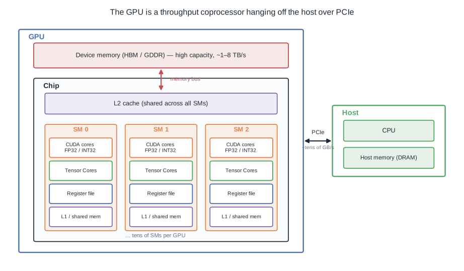
At the top level there are two separate worlds connected by a straw:

• The host — your CPU and its DRAM. This is where the process lives, where kernels are launched, and where data starts.
• The device — the GPU, with its own high-bandwidth memory (HBM/GDDR delivering 1–8 TB/s) feeding a chip full of compute.
• The PCIe link between them moves only tens of GB/s. That asymmetry — TB/s on-device vs GB/s across PCIe — is the single most common source of “my GPU is idle” surprises.

Inside the chip: a large shared L2 cache in front of HBM, and an array of Streaming Multiprocessors (SMs). The SM is the unit that actually executes your code.

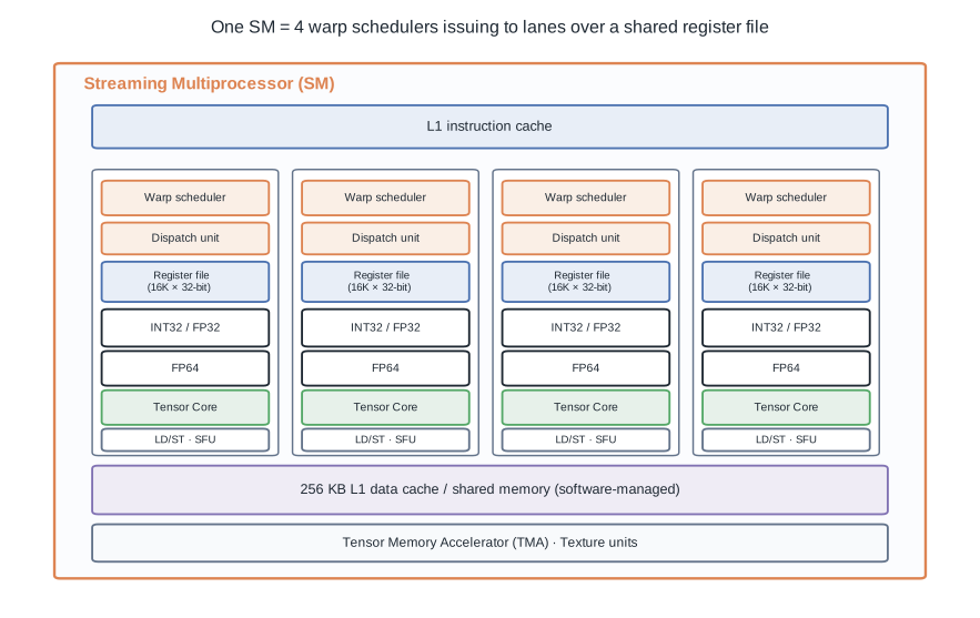
An SM is partitioned into a handful of processing blocks, each with its own warp scheduler and dispatch unit, feeding lanes of INT32/FP32/FP64 units and Tensor Cores, all backed by a big register file and a slab of L1 / shared memory. The critical detail: the register file and shared memory are finite and shared among every warp resident on the SM. How many warps you can keep resident — the occupancy — is decided by how greedily each thread consumes registers and shared memory. This is why “use fewer registers” is a real optimization and not folklore: it buys you more concurrent warps to hide latency with.

2. The Execution Model Exists to Hide Latency

CUDA’s hierarchy looks like bookkeeping. It is actually the mechanism that makes a memory-bound machine fast.

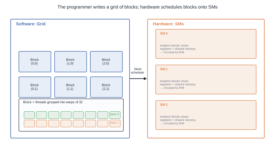
• You launch a grid of blocks. Each block is a group of threads that can share memory and synchronize with __syncthreads().
• Hardware chops each block into warps of 32 threads that execute the same instruction in lock-step (SIMT).
• The block scheduler assigns whole blocks to SMs. A block stays resident until it finishes.

The point of oversubscribing an SM with many warps is latency hiding. When a warp issues a global-memory load and stalls for hundreds of cycles, the scheduler instantly switches to another ready warp. With enough warps in flight, the memory latency disappears behind useful work. A kernel with low occupancy has nothing to switch to, so the SM sits and waits on HBM.

This model has one sharp edge — warp divergence — which we return to in §5.

3. The Memory Hierarchy Is the Whole Game

If you remember one figure, remember this one.

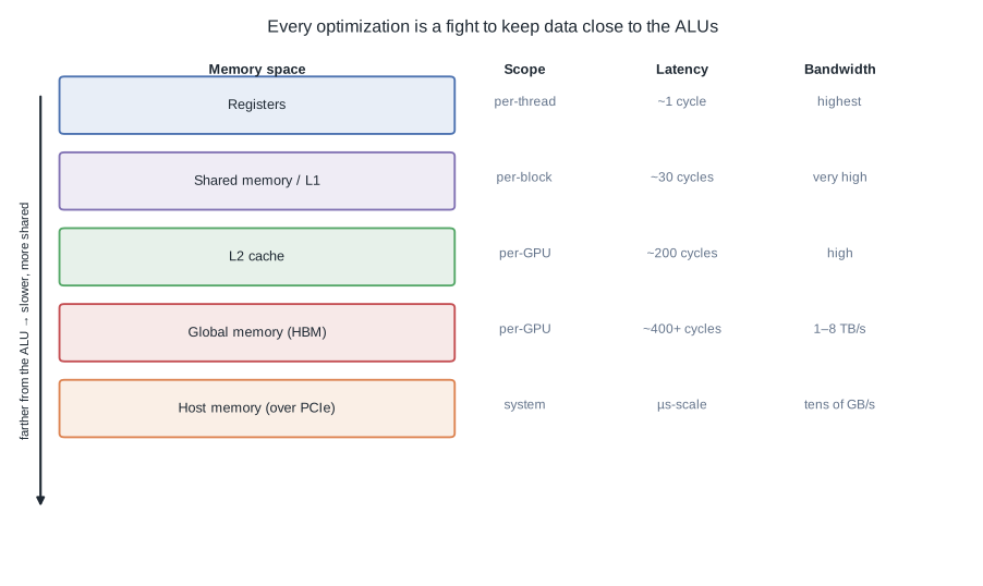
Each level down is dramatically slower and more shared than the one above it. A register access is essentially free; an HBM miss can cost 400+ cycles. The entire optimization catalog is a set of strategies for serving each byte from the highest level of this hierarchy that you can arrange.

That reframing is what turns a pile of tricks into three questions you can ask any hot kernel:

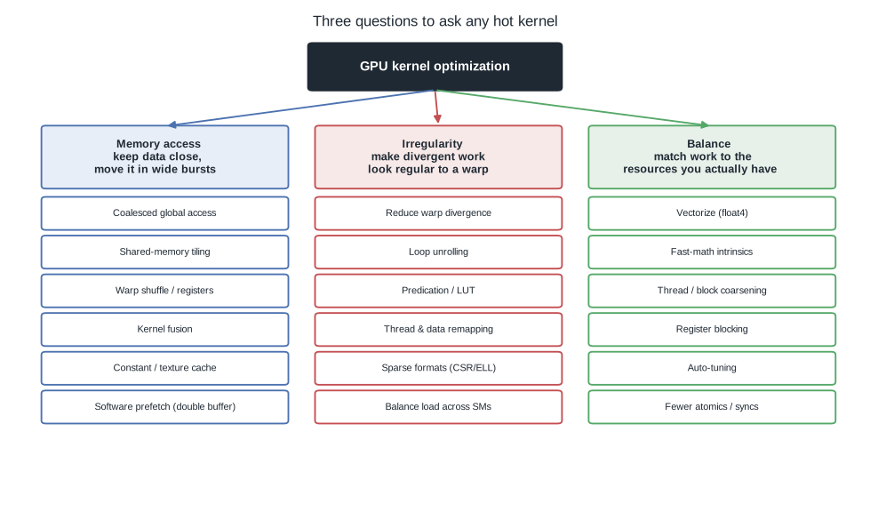
1. Memory access — is data as close to the ALUs as it can be, and am I moving it in wide, contiguous bursts?
2. Irregularity — is divergent or scattered work forcing the warp to do redundant or serialized work?
3. Balance — am I matching the amount of work per thread to the registers, bandwidth, and parallelism I actually have?

The rest of the post walks these three pillars.

4. Pillar 1 — Memory Access

Coalesce global loads

Global memory is delivered in aligned segments, not per-element. When the 32 threads of a warp read 32 contiguous addresses, the hardware fuses them into one transaction. Scatter those same accesses and you pay for many transactions, most of whose bytes you throw away.

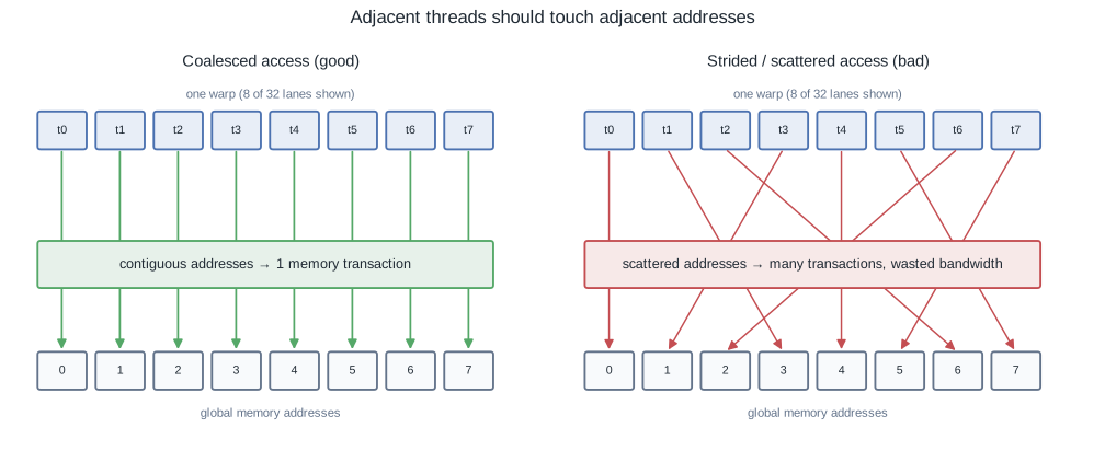
The rule is simple to state and easy to violate: make threadIdx.x map to the fastest-varying memory dimension. Row-major matrices want threads striding across columns, not rows.

1
2
3

// Coalesced: neighboring threads -> neighboring addresses.
int col = blockIdx.x * blockDim.x + threadIdx.x;
out[row * N + col] = in[row * N + col];  // one wide transaction per warp

Reuse through shared memory (tiling)

If a value is read by many threads, read it from HBM once into shared memory, then let the block hammer it at ~L1 speed. Tiled GEMM is the canonical example: stage tiles of A and B into shared memory, and the arithmetic intensity of the kernel climbs from “memory-bound” to “compute-bound.”

1
2
3
4
5
6
7
8
9

__shared__ float As[TILE][TILE], Bs[TILE][TILE];
for (int t = 0; t < N / TILE; ++t) {
    As[ty][tx] = A[row * N + (t * TILE + tx)];
    Bs[ty][tx] = B[(t * TILE + ty) * N + col];
    __syncthreads();                 // tile is now resident for the whole block
    for (int k = 0; k < TILE; ++k)
        acc += As[ty][k] * Bs[k][tx];
    __syncthreads();
}

Two caveats that separate a working tiled kernel from a fast one:

• Bank conflicts. Shared memory is split into 32 banks. If lanes in a warp hit the same bank on different rows, accesses serialize. The classic fix is padding the leading dimension ([TILE][TILE + 1]) so the stride skips the conflict.
• Warp-level reuse without shared memory. For reductions and small exchanges, __shfl_sync() moves data directly between registers of a warp — no shared-memory round trip, no __syncthreads().

1
2
3

// Warp reduction entirely in registers.
for (int off = 16; off > 0; off >>= 1)
    val += __shfl_down_sync(0xffffffff, val, off);

Fuse kernels to cut round-trips

Every separate kernel writes its output to HBM and the next kernel reads it back. A chain like matmul → bias → GELU as three kernels pays three HBM round-trips on the same tensor. Fusing them keeps the intermediate in registers and touches HBM once. This is exactly the win that torch.compile and FlashAttention monetize — fewer launches, less traffic.

Prefetch and specialized caches

• Software prefetch / double buffering: while computing on the current tile, issue the loads for the next tile so transfer latency overlaps compute.
• Constant memory: small, read-only, broadcast data (coefficients, small weights) is cached and served to a whole warp in one shot.
• Texture / read-only cache: good for 2D spatial locality and irregular read-only access.

5. Pillar 2 — Irregularity

Regular, dense work maps beautifully onto SIMT. Real workloads are lumpy, and the lumps cost you.

Warp divergence

Because a warp shares one program counter, a data-dependent branch forces the hardware to run both sides, masking off the inactive lanes on each pass. A balanced if/else inside a warp can halve throughput.

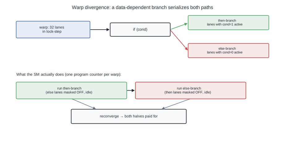
Mitigations, in rough order of preference:

• Restructure so a branch aligns with warp boundaries — if all 32 lanes take the same side, there is no divergence.
• Predication for tiny branches: compute both cheap results and select, avoiding a real branch.
• Lookup tables to replace branchy logic with a memory read.
• Thread / data remapping (e.g. sorting or compaction) so similar work lands in the same warp.

Load imbalance and sparsity

If some blocks finish early while others grind on, SMs idle. Uneven work — sparse matrices, ragged batches, variable-length sequences — needs either better data structures (CSR/ELLPACK/COO for sparse matrices pack the nonzeros and regularize access) or dynamic remapping so each warp gets comparable work.

Loop unrolling

Unrolling (#pragma unroll) cuts loop overhead and exposes independent instructions, improving instruction-level parallelism and giving the scheduler more to overlap. It trades registers for speed, so it interacts with occupancy — measure, don’t assume.

6. Pillar 3 — Balance

Once data is close and warps are regular, the remaining game is matching the amount of work to the hardware.

Balance the instruction stream

• Vectorize. Load and store float4/int2 so one instruction moves 128 bits. Fewer, wider memory instructions raise effective bandwidth — when alignment allows it.
• Fast-math intrinsics. __sinf, __expf, __fdividef trade a few ULPs of accuracy for far higher throughput. Fine for many ML workloads, dangerous for numerics that need it.
• Warp-centric programming. Design around the warp as the unit (shuffles, ballots, warp-level primitives) rather than fighting the SIMT model thread-by-thread.

Balance parallelism

• Thread / block coarsening. Sometimes fewer threads each doing more work wins: it amortizes launch and index overhead and improves register reuse. The naive “one thread per output element” is often not optimal.
• Register blocking. Have each thread compute a small tile of outputs held in registers, maximizing reuse of operands already loaded.
• Auto-tuning. Block size, tile size, and unroll factor interact non-linearly with occupancy. The right values are hardware- and shape-specific; sweep them (this is exactly what Triton’s autotuner and CUTLASS do).

Balance synchronization

• Fewer __syncthreads(). Barriers stall the whole block; hoist or eliminate the ones you can.
• Fewer atomics. Contended atomics serialize. Prefer hierarchical reductions (warp → block → grid) that atomically combine only partial results.
• Cross-block coordination via Cooperative Groups when you genuinely need grid-wide sync, instead of splitting into extra kernels.

7. Where to Actually Start

The catalog above is a menu, not an itinerary. Ordering matters more than completeness:

1. Profile first. Nsight Compute or the PyTorch profiler tells you whether you are compute-bound or memory-bound. The Roofline model turns that into a target. Optimizing in the wrong direction is the most expensive mistake in performance work — see Roofline: The First Step of Any Performance Optimization.
2. Fix the binding constraint. Memory-bound? Coalesce, tile, fuse. Compute-bound? Tensor Cores, lower precision, better tiling. Don’t unroll a loop in a kernel that is waiting on HBM.
3. Reach for libraries before PTX. For the overwhelming majority of workloads, torch.compile, FlashAttention, cuBLAS, and CUTLASS already encode more of this playbook than you will hand-write. Custom kernels earn their keep only where a profiler proves a real, fusible gap.

The three questions — is data close? is work regular? is it balanced? — are enough to reason about almost any kernel without memorizing the trick list. The tricks are just the answers.

References

- Hijma, Heldens, Sclocco, van Werkhoven, Bal, Optimization Techniques for GPU Programming, ACM Computing Surveys 55(11), Article 239, 2023 — the 450-paper survey behind this post’s three-pillar taxonomy.
- Williams, Waterman, Patterson, Roofline, CACM 2009; NVIDIA CUDA C++ Programming Guide and DL Performance Guide
- Dao et al., FlashAttention; Horace He, Making Deep Learning Go Brrrr