Data Parallelism: From Parameter Server to Ring All-Reduce
Data parallelism is the default scaling move because it preserves the model program. Every rank owns the same model, sees different examples, computes gradients, and applies the same update.
The algorithm is simple. The system is not. The whole post is about removing one bottleneck: do not push all gradient traffic through one server when every GPU could be moving bytes at the same time.
Parameter servers made large-scale training practical for many early workloads (OSDI 2014). Ring all-reduce made dense synchronous training scale cleaner on GPU clusters; Baidu’s deep learning systems work and Horovod were the public turning points for many practitioners (arXiv:1702.05847, arXiv:1802.05799). PyTorch DDP wraps the same collective contract around autograd buckets (arXiv:2006.15704).
TL;DR
- Data parallelism shards the batch, not the model. Each rank keeps a full model replica.
- Synchronous DP requires every rank to apply the same reduced gradient. That invariant is the contract.
- A parameter server is easy to reason about, but one server link sees traffic from all workers.
- Ring all-reduce decomposes all-reduce into reduce-scatter plus all-gather. For
Mbytes acrossNranks, per-rank traffic is2 * (N - 1) / N * M. - PyTorch DDP overlaps gradient all-reduce with backward by launching collectives when gradient buckets become ready.
- Ring is bandwidth-efficient for large buckets, not latency-optimal for tiny tensors. Bucketing is part of the algorithm, not an implementation detail.
- Plain DDP does not solve model-state memory. ZeRO/FSDP exists because every DP rank still stores parameters, gradients, and optimizer state.
- Reproducible figures for this post:
playground/llm_training_series_figures.py.
1. The Contract
Let a model have parameters W. Split the global batch across N workers. Worker i computes a local gradient G_i.
Synchronous data parallelism computes:
Every rank applies the same update. If replicas diverge, the run is no longer ordinary synchronous data parallel training.
This contract survives many implementation choices:
- Centralized or decentralized communication.
- Full-gradient all-reduce or bucketed reductions.
- All-reduce or reduce-scatter plus sharded optimizer.
- Communication after backward or overlapped with backward.
The reason DP is popular is that the model code barely changes. The expensive part is now gradient synchronization.
The reason DP stops scaling is equally direct: every rank stores the full parameter set, full gradients, and optimizer state unless another method shards them. That is why the next post moves to ZeRO.
2. Parameter Server: Simple, Centralized, Hot
The parameter-server design separates workers from servers that own parameters, gradients, or optimizer state.
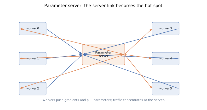
A synchronous loop:
- Workers hold model replicas.
- The input batch is split across workers.
- Workers compute local gradients.
- Workers push gradients to the server.
- The server aggregates gradients and updates parameters.
- Workers pull updated parameters.
This design is flexible. It supports sparse updates, custom consistency models, CPU-backed state, and sharded parameter placement. The OSDI 2014 parameter-server paper was built for that wider distributed ML world, not only dense Transformers (OSDI 2014).
The failure mode is load concentration. With one server and dense gradients of size M, the server handles roughly:
| |
Workers are mostly waiting on the server link. Adding more workers increases the server’s traffic. Sharding across multiple servers reduces the hot spot, but now placement and consistency become system design problems.
For dense GPU training, where every layer produces dense gradient tensors and every rank needs the same update, collectives are the cleaner fit.
3. Async SGD: More Utilization, Stale Gradients
Synchronous training waits. One slow worker delays the step. Asynchronous SGD removes some waiting by letting workers push gradients computed from older parameter versions.
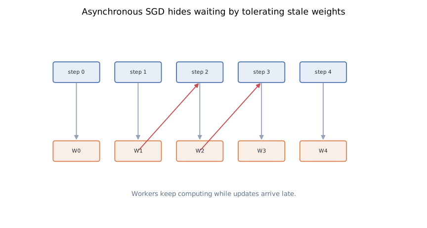
The benefit is hardware utilization. Workers do not have to idle at a global barrier.
The cost is staleness:
Stale gradients can still converge under bounded assumptions, but the optimizer is no longer the same as synchronous mini-batch SGD. Tuning becomes system-dependent. Fast workers can dominate update frequency; slow workers may contribute gradients from old weights.
Modern dense LLM pretraining usually chooses synchronous DP because Transformer compute is regular, collectives are optimized, and reproducibility matters. Async and bounded-staleness designs remain useful for sparse recommenders, elastic training, and parameter-server workloads. They are not the default dense LLM path.
4. DDP: Keep Semantics, Replace the Server
Distributed Data Parallel keeps the synchronous DP contract and replaces the server with collective communication.
In PyTorch DDP, each process owns one model replica. During backward, autograd hooks mark gradients ready. DDP groups parameters into buckets. When a bucket is ready, it launches a reduction for that bucket, overlapping communication with the remaining backward compute (PyTorch DDP docs, arXiv:2006.15704).
Conceptually:
The all-reduce must produce the same reduced gradient on every rank. A gather-to-one-rank implementation would recreate the parameter-server bottleneck. Ring all-reduce distributes the traffic.
5. Ring All-Reduce = Reduce-Scatter + All-Gather
Assume N ranks in a logical ring and a gradient tensor of size M. Split the tensor into N chunks of size M/N.
The first phase is reduce-scatter.
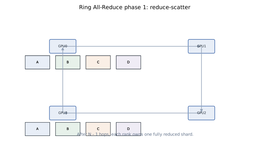
At each step, every rank sends one chunk clockwise and receives one chunk counter-clockwise. The received chunk is added into a local partial sum. After N - 1 steps, every rank owns one fully reduced chunk.
Rank-local send volume for reduce-scatter:
| |
No rank is special. Every rank sends and receives the same amount at every step. This is the core load-balance difference from a single parameter server.
The second phase is all-gather.
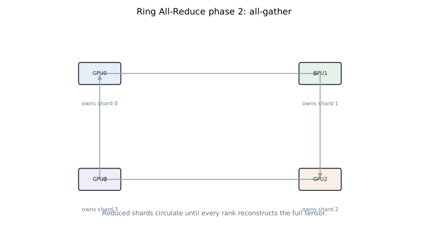
Each rank forwards already-reduced chunks until every rank has the full reduced tensor. The send volume is the same:
| |
Total per-rank traffic:
| |
For large N, this approaches 2M. That is the practical “two tensor transfers” rule for dense ring all-reduce.
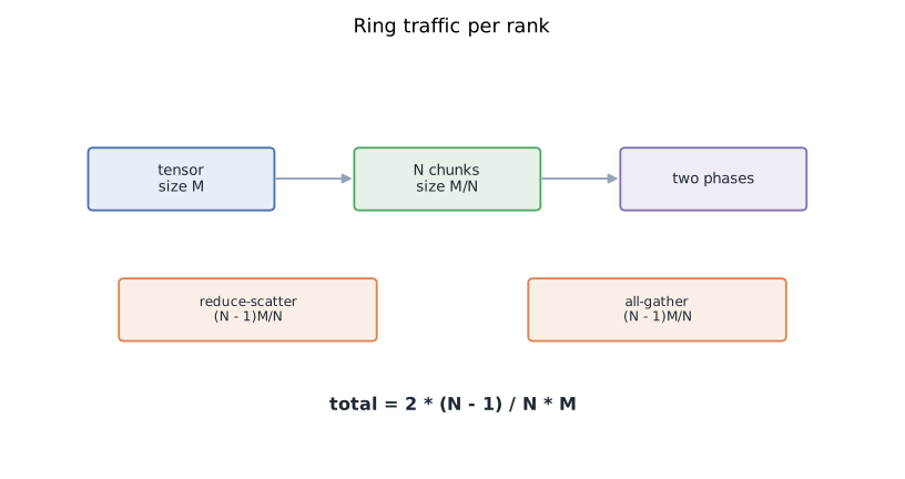
The bandwidth formula is older than deep learning; Patarasuk and Yuan formalized bandwidth-optimal all-reduce algorithms for clusters (JPDC 2009). Baidu’s work showed the same HPC-style collective thinking was decisive for deep nets on GPU clusters (arXiv:1702.05847).
6. Why Ring Works for Big Buckets
Ring is not universally best. It takes 2(N - 1) communication steps, so tiny tensors can be latency-bound.
For large gradient buckets, ring has the right shape:
- Every rank is active.
- Transfers are large and contiguous.
- No central link carries all traffic.
- Per-rank bandwidth cost is close to optimal for large payloads.
This is why DDP buckets gradients. One all-reduce per parameter tensor would drown in latency. One giant bucket would reduce overlap because early gradients would wait for late gradients. The bucket size is a real performance knob.
NCCL may choose rings, trees, CollNet, or topology-aware mixtures depending on message size and hardware. The ring model is still worth learning because it explains the reduce-scatter/all-gather decomposition that also appears in ZeRO and distributed optimizers.
7. What DDP Still Does Not Solve
DDP removes the central communication hot spot for synchronous dense training. It does not remove memory redundancy.
With mixed precision Adam, a common static model-state budget is roughly:
Plain DDP puts that on every rank. A 70B parameter model would require about 1.12 TB of model-state memory per replica before activations. No all-reduce trick fixes that.
DDP also does not remove stragglers. One slow rank delays the synchronized step. It does not automatically choose topology-aware process groups. It does not make gradient buckets large enough or small enough for your model. Those are job-level engineering responsibilities.
This is why real LLM training stacks compose DDP-style semantics with ZeRO, tensor parallelism, pipeline parallelism, sequence parallelism, and communication overlap.
8. Practical Debugging Checks
When a DDP job underperforms, check these before changing the model:
- Global batch math: each rank receives the intended local batch, and loss scaling matches gradient averaging.
- Bucket timing: all-reduces should start during backward, not only after backward completes.
- Bucket size: tiny buckets waste latency; huge buckets delay overlap.
- Unused parameters: dynamic graphs can force extra graph traversal or missing-gradient handling.
- Stragglers: data loading, variable sequence length, thermal throttling, or one bad node can dominate a synchronous step.
- Topology: rank order should respect NVLink/NVSwitch islands, PCIe layout, and cross-node fabric.
- Precision: gradient dtype and communication hooks change both bandwidth and numerical behavior.
DDP is not just an API. It is a communication schedule attached to autograd.
9. Code
The best code to read:
- PyTorch
DistributedDataParallel: bucket setup, autograd hooks, reducer integration, and user-facing DDP behavior. - PyTorch c10d: process groups and collective backends.
- PyTorch distributed package: Python API surface around process groups, collectives, and launch utilities.
- Horovod: ring-allreduce-centered distributed training across TensorFlow, PyTorch, and MXNet.
- NCCL: production GPU collectives. You rarely read it first, but it is the layer that often decides actual all-reduce performance.
Trace one gradient bucket from “autograd produced these grads” to “all ranks have the reduced bucket.” That path explains most DDP performance bugs.
10. Minimal Mental Model
Keep three invariants:
Data parallelism is the cleanest throughput axis while a replica fits. Once the replica does not fit, the next move is not a better all-reduce. It is sharding the redundant state.
References
- Mu Li et al., Scaling Distributed Machine Learning with the Parameter Server, OSDI 2014.
- Andrew Gibiansky et al., Bringing HPC Techniques to Deep Learning, 2017.
- Alexander Sergeev and Mike Del Balso, Horovod: Fast and Easy Distributed Deep Learning in TensorFlow, 2018.
- Shen Li et al., PyTorch Distributed: Experiences on Accelerating Data Parallel Training, VLDB 2020.
- Pitch Patarasuk and Xin Yuan, Bandwidth Optimal All-reduce Algorithms for Clusters of Workstations, Journal of Parallel and Distributed Computing, 2009.
- Sixin Zhang et al., Poseidon: An Efficient Communication Architecture for Distributed Deep Learning on GPU Clusters, 2017.
- Awni Hannun et al., Deep Speech: Scaling up end-to-end speech recognition, 2014.
- Code and docs: PyTorch DDP docs, PyTorch DDP code, PyTorch c10d, Horovod, NCCL.